I built an interactive map that visualizes employment flows across the United States, where people live and where they work. The data comes from the Census Bureau's LODES dataset, which tracks origin-destination employment at the census block level for 95% of US jobs.
A quick note on what "flows" means here: LODES records where someone lives and where their job is. For neighboring counties that's a literal daily commute. But the data also includes things like someone living in Hawaii and working in New York, which isn't a daily drive, it's probably remote work or seasonal employment. So this is really a map of employment connections, not strictly commutes. The road routing still makes sense for the vast majority of pairs though since most flows are between nearby counties.

The final result: click any county and watch employment flows light up along actual highway corridors, animated across 22 years (2002-2023). You can toggle between arc view and road-snapped view. The frontend is deck.gl on a dark map, deployed as a static site on Cloudflare Pages.
from billions of records to 280k pairs
LODES (LEHD Origin-Destination Employment Statistics) provides block-to-block employment data, where a worker lives and where they work, broken down by age, earnings, and industry. I used the LODES8 release covering 2002-2023.
The raw data is massive. Each state has two OD files per year:
od_mainfor when both home and work are in-stateod_auxfor when work is in-state but home is out-of-state
Plus a crosswalk file that maps census blocks to counties, tracts, CBSAs, etc. Across 51 states and 22 years, that's over 14 million rows of county-level aggregated data.
Here's how the data funnels down:
- Raw LODES: billions of census block-to-block records (e.g., "3 people live in block 060371234001 and work in block 170318765002")
- County aggregation: each census block maps to a county via the crosswalk, so all those block-level records roll up into county-to-county pairs. "Block A to Block B: 3 jobs" becomes part of "LA County to Cook County: 1,247 jobs"
- Result: ~823k unique county pairs across 3,144 counties, 146 million total job-years tracked
- Filtered for the web (pairs where at least 10 people commuted in any year): 280k pairs
- Road-routed (pairs with actual highway geometries): 96k pairs
The data isn't lost at each step, it's summed. Those billions of block records are all contained in the 280k county pairs, just aggregated up. A single pair like "San Bernardino County to LA County" represents tens of thousands of individual block-to-block commute records.
All processing is done with polars in Python. The crosswalk files have fun surprises like sentinel values (9999999999999999999999) that overflow i64, and mixed-type columns like 4665R in a numeric field. I ended up using infer_schema=False to read everything as strings and casting later.
straight lines are boring
The first version used deck.gl's ArcLayer, curved lines from home county to work county. It worked but it looked generic.
I saw busrouter.sg and got inspired by their stacked PathLayer look, thin green lines elevated off the map surface, layered on top of each other. The key things I learned from their code: each route gets a unique "level" so overlapping routes stack at different heights, depthTest: false is critical for the layered look, and blend: true handles the transparency compositing.
It looked way better but the lines were still straight. A flow from Orange County to LA showed as a diagonal line cutting through the mountains instead of following the 5 Freeway. The whole point is seeing which highways light up.
so I used OSRM to route the flows
OSRM (Open Source Routing Machine) is a routing engine that runs on OpenStreetMap data. You give it two coordinates and it returns the actual road path between them. It's free, open source, and you can self-host it.
The plan: pre-compute road-snapped routes for all 96k county-to-county pairs, save the polylines as static JSON, and render them on the frontend. No routing at runtime. This ended up taking four attempts.
attempt 1: public OSRM server
OSRM runs a public demo server at router.project-osrm.org. I wrote an async Python script with httpx to query it, save progress every 50 routes so it could resume if interrupted.
It immediately started returning connection refused. The public server was down at the time.
attempt 2: self-host full US
OSRM needs to preprocess the road network before it can route. You download the OSM extract, run osrm-extract, osrm-partition, osrm-customize, then start the server.
I downloaded the full US extract from Geofabrik and ran osrm-extract in Docker:
docker run -t -v "${PWD}:/data" osrm/osrm-backend \
osrm-extract -p /opt/car.lua /data/us-latest.osm.pbf
It died. Exit code 137, OOM killed. I bumped Docker's memory to 16GB. Died again. The full US extract needs ~50GB+ RAM for preprocessing.
There's also another problem: the OSRM Docker image is x86-only. On Apple Silicon, Docker emulates through Rosetta which adds significant memory overhead on top of the already massive requirements.
attempt 3: state-by-state
I downloaded just California from Geofabrik (~1.2GB). This time osrm-extract finished in under a minute and the peak RAM was 6.8GB. Partition and customize also went through fine.
Started the server, tested it:
curl -s "http://localhost:5000/route/v1/driving/-118.24,34.05;-117.16,32.72?overview=simplified&geometries=geojson"LA to San Diego, routed through actual roads. Then I ran all 96k flows through it at 637 routes/sec.
The problem: the California OSRM server only had California roads. So routes like NYC to New Jersey got snapped to random California roads, which is obviously garbage.
So the plan became: download each state's extract, process OSRM, route only that state's in-state flows, tear down, move on. I even wrote a bash script that automated the whole loop, download, extract, partition, customize, start server, route, stop Docker, clean up, next state. But then I realized the visually interesting flows are the cross-state ones. NJ to NYC. Maryland suburbs to DC. The I-95 corridor. State-by-state misses the whole point.
I also briefly considered the Mapbox Directions API (100k free requests/month, which would cover our 96k routes), but their ToS doesn't allow caching route geometries for display outside Mapbox maps. Since we're pre-computing and storing routes as static files, that's a violation.
attempt 4: highway-only US extract
The key insight: for county-to-county flow visualization, we don't need every residential street and parking lot. We just need highways.
osmium-tool can filter OSM data by tags:
osmium tags-filter us-latest.osm.pbf \
  w/highway=motorway,trunk,primary,secondary \
  -o us-highways.osm.pbf
This strips everything except motorways, trunk roads, primary, and secondary roads. The file went from 10GB to 288MB. A 97% reduction.
OSRM processed it without breaking a sweat. The routing server handled all 96k pairs in under 3 minutes at 637 routes/sec with 50 concurrent workers.
The only pairs that fail to route are ones that require ferry crossings or ocean crossings. Alaska, Hawaii, and some Washington state Olympic Peninsula counties. About 460 pairs total. Every road-connected county pair in the continental US has a route.
workforce choropleth: where are the jobs?
After the commute flows page was done I wanted to do more with the LODES data. The origin-destination files tell you who goes where, but LODES also publishes RAC (Residence Area Characteristics) and WAC (Workplace Area Characteristics) files that tell you the totals: how many jobs are physically located in a county, and how many workers live there.
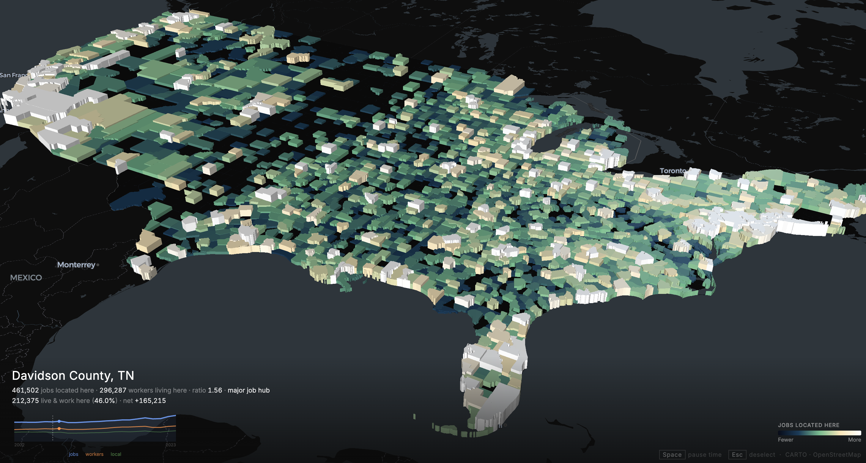
So I built a second page, a 3D choropleth where every county in the US is colored and extruded based on its workforce characteristics. You can switch between five metrics:
- WAC: total jobs located here
- RAC: total workers who live here
- Ratio (WAC÷RAC): above 1 means job hub, below 1 means bedroom community
- Net (WAC−RAC): positive means the county imports workers, negative means it exports them
- Retention: share of local jobs held by people who also live in the county
The pipeline downloads RAC and WAC files for all 51 states across 2002-2023, joins them to county FIPS via the crosswalk, and aggregates. The "local" metric comes from the existing OD data, it's the diagonal: people whose home county and work county are the same.
Check it out at where.putt.studio.